Hedge Accounting [Part 2]: Prospective Testing and the Risk Induced Fair Value

Photo by Jeff Fan on Unsplash - Downloaded on 16 June 2020
In the first part of this publication [Part 1], the importance of prospective testing was emphasised by summarizing and commenting the regulatory requirements of IFRS 9. The prospective classification into effective and ineffective hedge relationships was also discussed.
In this second part, a practical application is presented, which
uses a quantitative dollar offset method that is based on the Risk Induced Fair Value ("RiFV").
Hedge effectiveness in the context of IAS 39 and IFRS 9
The idea of the procedure presented is to reconcile prospective effectiveness testing on the basis of a sensitivity ("Sen") analysis with retrospective effectiveness testing, which is currently used widely in financial institutions. The approach follows the General approach outlined in IFRS 9[1], which allows financial institutions to continue accounting according to IAS 39. In addition, the so-called RiFV (see Figure 1) serves as the basis for measuring effectiveness.
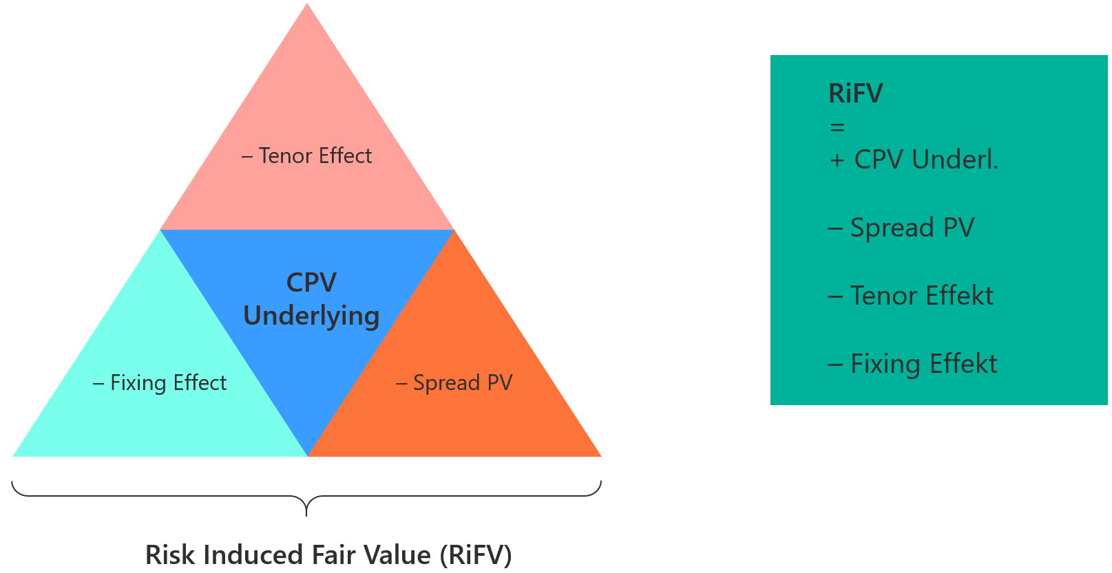
Figure 1: The RiFV as a fair valuation of an underlying that was hedged with a hedging transaction.
Effectiveness ratio (dollar offset method according to IAS 39):
The dollar offset method is used to test the effectiveness of a hedge relationship. This method considers the ratio of changes in the fair value of the hedged item and the changes in the fair value of the hedging instrument assigned to the hedged item. The effectiveness quotient provides information on the effectiveness of the hedge relationship on a quantitative basis. If the effectiveness is within a range of 80% to 125%, the hedge relationship is considered highly effective and hedge accounting can be applied subject to the other regulatory requirements (see Figure 2).

Figure 2: The quantitative Dollar Offset Method
The approach presented here introduces the dollar offset method, which can be realised on the basis of a sensitivity analysis. Two sensitivities of a) the RiFV (underlying transaction) and b) the hedging Transaction (see Figure 3) induced by a parallel shift of one basis point ("bp") of the yield/discount curve are calculated by building the quotient
Effectiveness = Sen RiFV Underlying / Sen Hedging Instrument.
The calculation of effectiveness based on the RIFV can be applied to both prospective and retrospective tests, but once in connection with sensitivities (in case of the prospective test) and once under consideration of past valuations (in case of the retrospective test).

Figure 3: Calculation of the sensitivities that are relevant for the effectiveness quotient: a) Underlying and b) Hedging Instrument, according to the RiFV Approach.
Introduction of the RiFV method
The basis for the RiFV is the clean present value ("CPV") of the underlying transaction ("U_CPV"). It is the present value ("PV") of all cash flows (Dirty PV "DPV") from the Underlying transaction ("U_DPV") adjusted for the accrued interest ("accruals"), which is the interest already accrued in the initial period containing the reference date of the assessment, from the start date of the period to the hedge start date or the as of date.
Since the effectiveness of the hedge relationship is limited solely to the hedging of the interest rate risk, the funding spread contained in the underlying transaction must be deducted for measuring the effectiveness of the hedge. This is usually done via the so-called Spread PV (“Sprd PV”), which is calculated based on the spread in the funding leg of the hedging transaction. To determine the Sprd PV, the difference between the CPV of the hedging instrument ("D_CPV") with spread and the D_CPV without spread is determined. In Addition to the Sprd PV, there is another effect, the Tenor Effect ("Tenor Eff") which must be taken into account. This effect should always be considered if the (risk-free) interest curves used for discounting have a different Tenor than the forward curves used to calculate the forward rates. There is a third effect, because the interest rate for the interest payment of the next interest period in the variable leg of a hedge is usually fixed at the beginning of the interest period. After the fixing date, the deviation of the variable interest rate from the previously fixed interest rate during the interest period results in ineffectiveness known as the Fixing Eff ("Fixing Eff"). In summary, the adjustments to the CPV of the hedged item described above result in the RiFV (see Table 1), on the basis of which the sensitivity of the hedged item can now be calculated (see Table 2).
| RiFV [with Optionality] | |
| = | |
| U_CPV [+ Swaption PV] | |
| – | |
| (Sprd PV [+ Swaption Sprd PV]) | |
| – | |
| (Tenor Eff [+ Swaption Tenor Eff]) | |
| – | |
| Fixing Eff |
When calculating the relevant sensitivities for the effectiveness measure from Table 2 and Table 3, a 1-bp parallel shift is implemented, i.e. the respective forward and Discount curves involved are shifted ("shftd") in parallel by +1-bp in absolute terms. Any dependencies between the curves must be resolved with the proposed procedure so that the shift of a curve has no effect on any dependent curves (e.g. EUR EONIA → GBP XOIS).
| Sen RiFV Underlying [with Optionality] | |
| = | |
| RiFV [with Optionality] (+1-bp shftd yield and discount curve) | |
| – | |
| RiFV [with Optionality] (non-shftd yield and discount curve) |
| Sen Hedging Instrument [with Optionality] | |
| = | |
| D_CPV [+ Swaption PV] (+1-bp shftd yield and discount curve) | |
| – | |
| (D_CPV [+ Swaption PV] (non-shftd yield and discount curve)) |
The sensitivity of the RiFV can alternatively be divided into four sub-sensitivities as shown in Figure 4:

Figure 4: Sensitivity of the Underlying according to the RiFV method - an alternative calculation
Finally, the calculation of the prospective effectiveness is introduced in Table 4.
| Prospective Effectiveness | |
| = | |
| Sen RiFV Underlying [with Optionality] | |
| / | |
| Sen Hedging Instrument [with Optionality] |
Example of a plain vanilla transaction
An actual example of the prospective effectiveness assessment[2] is illustrated below using a "plain vanilla" MM-transaction.
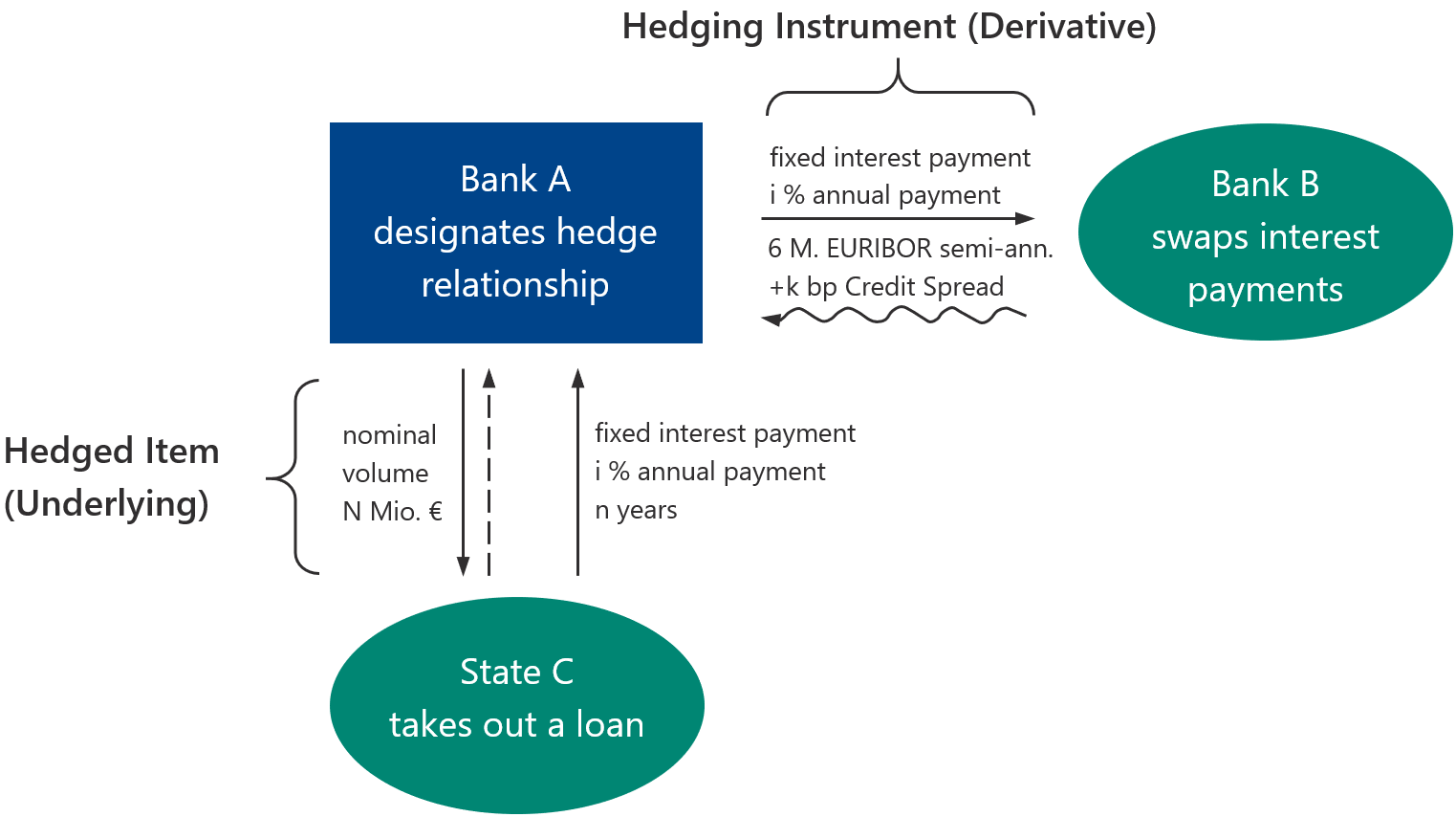
Figure 5: General example of a plain vanilla transaction from the perspective of Bank A: hedging the interest rate risk of a loan with a nominal value of N million EUR over the entire term of n years by means of an interest rate swap.
In the Underlying transaction Bank A lends State C the amount of EUR 25,564,594 (nominal) on 18 December 2003 with a maturity on 12 January 2028 at an annual interest rate of 6.185 %. Furthermore, on 1 October 2013 (hedge start date), the lender designates (assigns) to this underlying transaction a derivative interest rate swap with the same maturity date as the underlying. The fixed interest rate of 6.185 % is transferred to the counterparty Bank B and the lender of the Underlying receives a variable interest rate based on the EO6M yield curve, this time not annual but semi-annual, including a spread of +6-bp. The procedure for determining the corresponding sensitivities according to the RiFV method and the subsequent determination of prospective effectiveness is shown below in two steps. To simplify the calculation, the determination of sub-sensitivities (based on Figure 4) is of primary importance.
I.) Sensitivity calculation of the (Underlying) RiFV
Observing the Underlying transaction at the beginning of the hedge relationship, i.e. on the hedge start date, the corresponding series of cash flows, discounted with the EONIA curve, yields a series of present values on the as of date (see Figure 6).


Figure 6: Cash flows and present values of a loan that starts on 18 December 2003 and is due on 12 January 2028. Nominal: EUR 25,564,594, interest rate: 6.185 % as of 1 October 2013 (at hedge start). A deviation of the values determined with Summit and Excel occurs due to numerical rounding.
The sum of these PVs corresponds in Summit to a U_DPV of EUR -39,508,496. This figure must still be adjusted by the accrued interest in the amount of EUR 1,141,956. The DPV adjusted for the accrued interest is the U_CPV and amounts to EUR 38,366,540. For the sub-sensitivity of the U_CPV, the CPV is shftd by +1-bp in the amount of EUR 38,325,801. This shftd U_CPV is calculated in the same manner as the non-shftd U_CPV before, with the only difference being that the variable EONIA discount curve contains a parallel shift of +1-bp. The sensitivity of the underlying transaction can now be calculated using the difference between the two previously determined CPVs
Sen U_CPV = U_CPV (+1-bp shift) – U_CPV (non-shftd
= EUR 38,325,801 – EUR 38,366,540
= EUR -40,738.
The associated hedging transaction contains a spread of 6-bp (see Figure 7), which must be taken into account in both the shftd and non-shftd form when calculating the RiFV of the underlying.

Figure 7: Interest rate swap as hedge for the plain vanilla MM in this example
As shown in Figure 8 below, the CPV (incl. spread) of the structured pay leg (non-shftd) amounts to EUR -19,923,484 and the CPV of the funding receive leg is EUR 8,194,304. The sum of the two CPVs is therefore EUR -11,729,180 and corresponds to the D_CPV of the entire hedging transaction. If the spread is eliminated, i.e. set to 0, and the PV calculation is performed again, the CPV of the hedging transaction reduces to EUR -11,926,392.

Figure 8: CPV calculation of the hedging instrument with a non-shftd forward and discount curve as of 1 October 2013 (at hedge start). Left side: The credit spread of +6-bp is included. Right side: The credit spread is eliminated.
In the RiFV calculation, the contribution of the spread, which is subtracted from the U_CPV in order to consider the unhedged funding spread, defines the Sprd PV. It is the difference between the two CPVs
(EUR -11,729,180) – (EUR -11,926,392) = EUR 197,211 (non-shftd).
To determine the sub-sensitivity caused by the Sprd PV, the calculation basis of the shftd form is determined in the same manner as the non-shftd form of the Sprd PV, but now by means of the relevant yield and discount curve shftd in parallel by +1-bp. In the funding leg, this affects the EO6M interest rate curve required to determine the forward rates and the EONIA discount curve, whereas in the pay leg, only the EONIA discount curve needs to be shftd. The CPV of the hedging instrument with spread and incl. shift is EUR -11,689,749 and the CPV of the hedging instrument without spread incl. shift is EUR -11,886,823 (see Figure 13). This Sprd PV shftd in parallel by +1-bp corresponds to the difference between the two CPVs
EUR -11,689,749 – (EUR -11,886,823) = EUR 197,074.
The sub-sensitivity of the Sprd PV amounts to
Sen Sprd PV = Sprd PV (+1-bp shift) – Spread PV (non-shftd) =
= EUR 197.074 – EUR 197.211 = EUR -138.
Because the forward rate is fixed, the Tenor Eff has no effect on the structured leg (see Figure 9). To calculate the Tenor Eff, it is enough to look at the corresponding CPVs of the funding leg. For the derivative swap, the forward rate in the funding leg is determined based on the EO6M index. The corresponding cash flows are discounted based on EONIA (with a different tenor to EO6M), resulting in a CPV of EUR 8,194,304.
The analogous conversion of the forward curve to EONIA (corresponds to ZOIS in the following figure) results in a CPV of EUR 7,335,250 and thus a difference of
EUR 7,335,250 – EUR 8,194,304 = EUR -859.054,
which corresponds to the non-shftd Tenor Eff.

Figure 9 Impact of the Tenor Eff as of 1 October 2013 (at hedge start). Graphic above: EO6M-Forward Rate. Graphic below: EONIA (ZOIS) forward rate. In this case, the Tenor Eff only affects the Funding (receive) leg and corresponds to 0 in the structured leg (red).
When calculating the Tenor Eff with a +1-bp shift, the funding legs' forward rate is first determined based on an EO6M forward curve shftd in parallel by +1-bp. The corresponding cash flows are discounted using the EONIA curve shftd in parallel by +1-bp. After the deduction of the accrued interest, the CPV of EUR 8,219,334 is obtained. Subsequently, the CPV for which the forward rates were formed using the ZOIS (EONIA) curve shftd in parallel by +1-bp must be subtracted from the previous calculated CPV. After discounting was carried out with the same tenor, i.e. using the EONIA curve, this CPV amounts to EUR 7,360,722.
The Tenor Eff with a shftd discount curve corresponds to the difference between the CPVs
Tenor Eff (+1-bp shift) = (EUR 7,360,722 – EUR 8,219,334) =
= EUR -858,612.
The sub-sensitivity of the Tenor Eff is
Sens Tenor Eff = (EUR -858,612) – (EUR -859,054) = EUR 442.
The Fixing Eff arises in the funding leg of the derivative due to the deviation of the interest rate of the 6-month EO6M (0.33%) fixed on 10 July 2013 for the interest period from 12 July 2013 to 13 January 2014 and the interest rate (0.1694%) expected on the as of date (hedge start) for the interest payment on 13 January 2014, which depends on the EO6M curve that is updated daily (see Figure 10 and Figure 11).

Figure 10: Cash flows with fixed interest period of the interest rate swap (funding leg) as of 1 October 2013
The Fixing Eff is now calculated by subtracting the PV of the accrued interest from hedge start until the end of the period (interest payment) under the fixed rate from the PV of the accrued interest under the moving daily forward rate at hedge start. Accordingly, in this example, the interest portion from 1 October 2013 to 13 January 2014 must be calculated with different rates and discounted using the present discount curve:


Figure 11: Calculation of the Fixing Eff as of 1 October 2013
With a non-shftd forward/discount curve, the Fixing Eff amounts to EUR 11,857. With the corresponding curves shftd in parallel by +1-bp (EO6M forward and EONIA discount curve), the Fixing Eff is EUR 11,133. The sensitivity of the Fixing Eff of the difference is thus
Sen Fixing Eff = (EUR 11,133) – (EUR 11,857.30) = EUR -724.
In the last row of Figure 12 below, the sensitivity of the RiFV can finally be determined by subtracting the respective previously determined partial sensitivities of Sprd PV (-138), Tenor (442) and Fixing Eff (-724) from the sensitivity of the U_CPV (-40,738).

Figure 12: Calculation of the RiFV as of 1 October 2013
The sensitivity of the RiFV can also be calculated analogously according to Table 2 using the difference of the RiFVs determined in Figure 11
Sen RiFV = RiFV (+1-bp shift) – RiFV (non-shftd) =
= 38,976,206 – 39,016,525 = -40,319.
I.) Sensitivity calculation of the Hedging Instrument D_CPV
Figure 8 shows the CPV of the structured leg without shift (EUR -19,923,484) and the CPV of the funding leg without shift (EUR 8,194,304). The corresponding CPVs, obtained with the interest rate and discount curve shftd in parallel by +1-bp, amount to EUR -19,909,083 for the structured leg and EUR 8,219,333.71 for the funding leg. This results in the aggregated CPVs of the Hedging Instrument
D_CPV (+1-bp shift) = (EUR 8,219,334 – EUR 19,909,083)
= EUR -11,689,749
and
D_CPV (non-shftd) = (EUR 8,194,304 – EUR 19,923,484)
= EUR -11,729,180.
Consequently, the sensitivity of the Hedging Instrument is
Sen D_CPV = D_CPV (+1-bp shift) – D_CPV (non-shftd) =
= (-11,689,749) – (-11,729,180) = 39,431.

Figure 13: Calculation of the D_CPV of the hedging instrument and its sensitivity as of 1 October 2013
Using the quotient of the sensitivities from I.) and II.), the effectiveness of the hedge relationship
Effectiveness = Sen RiFV / Sen Hedging Instrument
= -40,319 / 39,431 = -1.02
is between -0.8 and -1.25 and thus the hedge is classified as prospectively effective according to the dollar offset method.
Practical implementation
The prospective effectiveness measurement could be manifested in an automated report (e.g. text or Excel file), which, for example, is generated daily and contains the prospective effectiveness of hedge relationships. By default, the effectiveness is determined at the beginning of the hedge on the basis of a mathematical process.
In addition to the RiFV method, the determination of prospective effectiveness can be achieved by several possible alternative approaches. For example, a variation in the shift (parallel vs. bucket, dependent vs. independent yield/discount curves) or the spread (Sprd PV, PV01, Sprd Schedule or an averaged Sprd) can be implemented (see Figure 15). The following table shows one possibility for calculating the RiFV (with PV01), which can be used in the linear case:
| RiFV | |
| = | |
| U_CPV | |
| – | |
| (EYS + FS) * PV01 | |
| – | |
| Tenor Eff | |
| – | |
| Fixing Eff |
where
Effective Yield Sprd (EYS): Additional margin if the hedge instrument is an effective yield swap.
Funding Sprd (FS): Initial credit margin of the hedge instrument + possible further effects.
PV01: Present value effect from a shift of one basis point for the underlying transaction's coupon. It is calculated by subtracting the PVs of a +1-bp coupon shift and without a coupon shift.
One way of accurately calculating the so-called (sub-)effectiveness of individual periods is to shift individual "buckets", i.e. generic points in time (e.g. 1M, 10Y, etc.) on the underlying yield/discount curve (see Figure 14). The number of buckets generally corresponds to the number of shifts, so that for each such bucket shift reflects a sub-sensitivity. In this manner, the sensitivities for the hedged item and the hedging instrument can be determined for a specific bucket and a (sub-)effectiveness can be determined for the respective period, indicating how prospectively effective the hedge was in this specific period. Due to the fixing at the beginning of the respective period, losses in effectiveness can occur, so that buckets that are hedged in this current period should be excluded from the effectiveness calculation.

Figure 14: Bucket shifts of an interest curve, orange 5 years, red 4 years and the aggregated interest curve in blue
When implementing individual variants, regulatory Framework conditions can leave a certain freedom in terms of the implementation. Depending on the risk management strategy pursued by the entity, the individual approach can be more or less accurate. Other simplified approaches can also be used to calculate sensitivities, such as a pure consideration of the CPVs of the underlying and a hedging transaction with eliminated credit spread ("CPV method"). This is done without consideration of the Sprd PV, Fixing and Tenor Eff.

Figure 15: Prospective effectiveness measurement: Modular structure of possible variations in the implementation
When implementing the method in a practical application, several special cases may occur, which must be taken into account according to their particularities. These include cross-currency transactions or the treatment of a changing hedge relationship. For example, various procedures can be defined individually for the selection of corresponding forward discount curves (FX sensitivities from shftd FX curves, translation at the closing rate after shifting the curves associated with the cash flows, etc.) depending on the circumstances and the risk strategy pursued when calculating the sensitivities.
In Summit, the individual cash flows are presented in a form where the end date of one period corresponds to the start date of the following period (see Figure 10). To avoid double consideration of interest days, it is therefore necessary to determine how these start and end dates are included in the cash flow calculation. Summit offers the option of a First Day Accrual method, in which the first day of a period is an interest day but the last day is not, and a Last Day Accrual method, in which the last day of a period is an interest day but the first day is not. It can be shown that the choice of the accrual method (First Day vs. Last Day accrual) has no influence on the amount of effectiveness according to the RiFV Dollar Offset Method presented here.
It is usually sufficient to assess the prospective effectiveness only once at the beginning of the hedge, if the hedge relationship designated to the underlying transaction remains unchanged until maturity.
Conclusion
The RiFV approach presented aims predominantly at the reconciliation of the prospective effectiveness measurement with the requirements for a quantitative retrospective effectiveness measurement in accordance with certain regulatory requirements. These requirements for the prospective test can be derived from the IAS 39 standard in the course of the used option[1] of IFRS 9 to perform hedge accounting according to IAS 39. The fundamental prospective effectiveness measurement realised via sensitivities is carried out based on the RiFV in order to subsequently apply a sensitivity analysis using the quantitative dollar offset method. This is performed for the balance sheet-relevant prospective classification into effective and ineffective hedging transactions. In addition to this proposed method for determining the prospective effectiveness, several different procedures for the determination of prospective effectiveness can be implemented, which, for example, allow for a variation in the shift (parallel, bucket) or the spread (Sprd PV, PV01, etc.).
Financial institutions are thus required to adopt a (risk) strategy which, in addition to the choice of a method that is in conformity with the regulations, weighs up the possibilities and Advantages of a more or less detailed implementation of the prospective test in order to be prepared during the ongoing extensive changeover to IFRS 9 and to be in line with the financial institution's Risk management strategy.
Our offer
The methods and solution approaches presented in this document allow for an extensive number of possible implementation strategies for a coherent prospective testing. We would be pleased to advise you in the context of a preliminary study in the analysis of possible solution variants of the effectiveness measurement and help you to develop the solution which, within the professional and technical possibilities, is adequately suited to the risk management strategy of your company.
Based on this, we can also assist you with the professional implementation.
For the implementation of individual solutions, our following core competencies provide significant benefits:
Quick, thorough and cross-sectoral process analysis and support,
Technical and professional know-how in hedge accounting and problem-solving,
Result orientation and integration ability in the development of systematic approaches.
We hope to have piqued your interest in our consulting services and we look forward to hearing from you.
References:
[1] Official Journal of the European Union, Commission Regulation (EU) 2016/2067 of 22 November 2016, IFRS 9: 7.2.22
[2] The calculations are presented with the precision of amounts rounded to euro.

![Hedge Accounting [Part 2]: Prospective Testing and the Risk Induced Fair Value](https://images.squarespace-cdn.com/content/v1/54f9ea6be4b0251d5319ad8b/1592205162143-L919DBQ2UQF59D4R9WFH/jeff-fan-29ebQh7e78M-unsplash.jpg)
![Hedge Accounting [Part 1]: Prospective Testing and the Risk Induced Fair Value](https://images.squarespace-cdn.com/content/v1/54f9ea6be4b0251d5319ad8b/1591683719107-BDZ43MTDO65RH9XKXBG6/christopher-burns-FUh6nK3s0po-unsplash.jpg)